Day 33

Math 216: Statistical Thinking

Bastola

Introduction to Categorical Data Analysis

Quantitative vs. Qualitative Data: Transition from numerical to categorical data, which includes discrete categories like opinions or health status.
Examples: Opinions range from Excellent to Poor; Health Status is either Sick or Healthy; Vaccination Status can be Yes or No.
Data Presentation: Often shown in tables counting occurrences across categories.

Categorical Data Representation

Table 1: Opinions on Pricing

Category	Observed
Pay much more	218
Pay somewhat more	497
Pay the same	425
Pay less	15

Table 2: Vaccination vs. Flu Status

Status	No Vaccine	One Shot	Two Shot	Total
Flu	24	9	13	46
No flu	289	100	565	954
Total	313	109	578	1000

Hypothesis Setup

Scenario: Evaluating gender distribution in a university STEM program against a regional expectation of a 50:50 male-to-female ratio.
Null Hypothesis (\(H_0\)): \(p_f = p_m = \frac{1}{2}\)
Alternative Hypothesis (\(H_a\)): \(p_f \neq p_m\)

Data Overview

Total Students: 500 (200 female, 300 male)
Expected under \(H_0\): Each gender = \(500 \times \frac{1}{2} = 250\)

Chi-Square Test Statistic

Test Statistic (\(T\)): A test statistic is one number, computed from the data, which we can use to assess the null hypothesis. Measures divergence of observed counts from expected counts under \(H_0\).
Calculation: Sum of the squared differences between observed and expected counts, normalized by expected counts.

\[\begin{aligned} \chi^2 = \sum{\frac{(observed - expected)^2}{expected}} = \sum{\frac{(O - E)^2}{E}} \end{aligned}\]

Chi-Square Distribution

Chi-Square Test Table

\[\begin{array}{|c|c|c|c|c|} \hline \textbf{Category} & \hat{p}_j & \textbf{Expected, } E_j & \textbf{Observed, } O_j \\ \hline \text{Female} & \frac{1}{2} & 250 & 200 \\ \hline \text{Male} & \frac{1}{2} & 250 & 300 \\ \hline \end{array}\]

Chi-Square Test Data Table

This table displays the categorical distribution of data for hypothesis testing.
- \(j\): Category index
- Category: Description of each category
- \(\hat{p}_j\): Estimated proportion for each category
- Expected, \(E_j\): Expected count under null hypothesis = \(n \hat{p}_j\)
- Observed, \(O_j\): Observed count in sample

\(j\)	Category	\(\hat{p}_j\)	Expected, \(E_j\)	Observed, \(O_j\)
1	\(\mathbf{C 1}\)	\(\hat{p}_1\)	\(n \hat{p}_1\)	\(n_1\)
2	\(\mathbf{C 2}\)	\(\hat{p}_2\)	\(n \hat{p}_2\)	\(n_2\)
\(\vdots\)	\(\vdots\)	\(\vdots\)	\(\vdots\)	\(\vdots\)
\(k\)	\(\mathbf{C k}\)	\(\hat{p}_k\)	\(n \hat{p}_k\)	\(n_k\)

Summary of the Steps

State Hypothesis
Calculate a test statistic, based on your sample data
Create a distribution of this statistic, as it would be observed if the null hypothesis were true
Measure how extreme your test statistic is, as compared to the distribution generated under null
Decision: Reject or fail to reject \(H_0\) based on the Chi-Square test value compared to critical values from Chi-Square distribution tables.
Implication: Determines if there is a statistically significant difference in gender distribution compared to regional expectations.

Example: Testing the Fairness of a Die

Outcome (Category)	1	2	3	4	5	6
Observed	12	7	14	15	4	8

Objective: Test whether the outcome of die rolls matches a fair die’s expected distribution.
Method: Use the Chi-Square test to compare observed outcomes against the expected frequencies for a fair die.

Testing the Fairness of a Die: R-code

# Assuming the die is fair, each of the 6 sides should appear with equal probability.
observed_counts <- c(12, 7, 14, 15, 4, 8)
expected_probabilities <- rep(1/6, 6)
chisq.test(x=observed_counts, p=expected_probabilities)


    Chi-squared test for given probabilities

data:  observed_counts
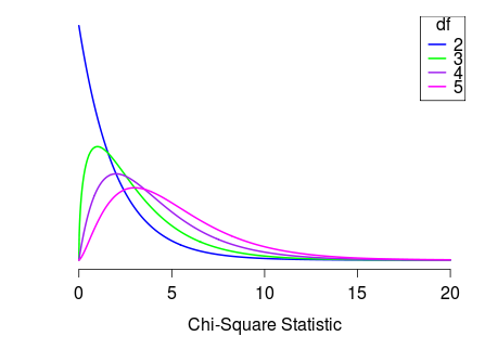
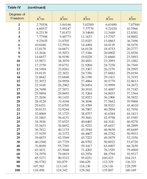
X-squared = 9.4, df = 5, p-value = 0.09413

Expected: Each side of the die should appear 10 times out of 60 rolls under the assumption of fairness.
Analysis: Perform the Chi-Square test and review the p-value to determine if there is significant evidence to reject the fairness assumption