Review of Simple Linear Regression Model Estimation
Recap: From the last session, we learned to estimate the simple linear regression line \(\hat{y} = \hat{\beta}_0 + \hat{\beta}_1 x\) from a sample.
Further Analysis Needs: To conduct deeper analysis, we adhere to key assumptions about the regression model.
Conducting a Simple Linear Regression
Step 1: Hypothesize the deterministic component of the model that relates the mean \(E(y)\) to the independent variable \(x\) (Section 11.2).
Step 2: Use the sample data to estimate unknown parameters in the model (Section 11.2).
Step 3: Specify the probability distribution of the random-error term and estimate the standard deviation of this distribution (Section 11.3).
Step 4: Statistically evaluate the usefulness of the model (Sections 11.4 and 11.5).
Step 5: When satisfied that the model is useful, use it for prediction, estimation, and other purposes (Section 11.6).
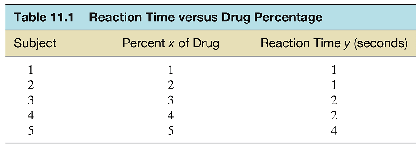
Example 1: Consider an experiment designed to estimate the linear relationship between the percentage of a certain drug in the bloodstream of a subject and the length of time it takes the subject to react to a stimulus. In particular, the researchers want to predict reaction time \(y\) based on the amount of drug in the bloodstream \(x\). Data were collected for five subjects, and the results are shown in Table 11.1. (The number of measurements and the measurements themselves are unrealistically simple in order to avoid arithmetic confusion in this introductory example.)
Step 1: Hypothesize the Deterministic Component
Focus: Straight-line models
Relationship: Mean response time to drug percentage
Assume the model relating mean response time \(E(y)\) to drug percentage \(x\):
\[
H: E(y) = \beta_0 + \beta x \longleftarrow \begin{aligned} & \text{The true unknown relationship} \\ & \text{between } x \text{ and } Y \text{ is a straight line} \end{aligned}
\]
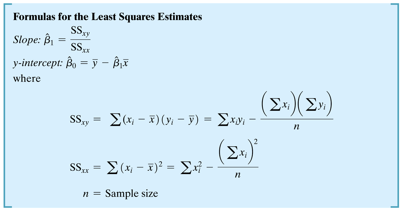
Step 2: Use sample data to estimate unknown parameters in the model.
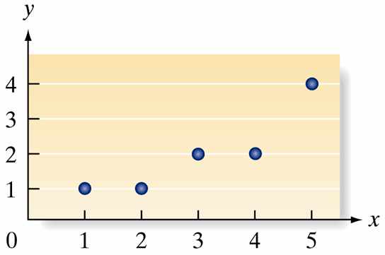
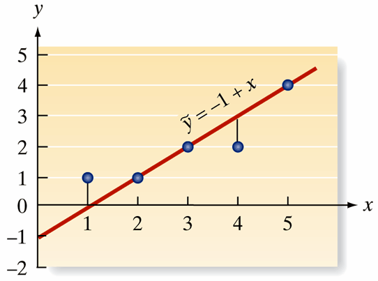
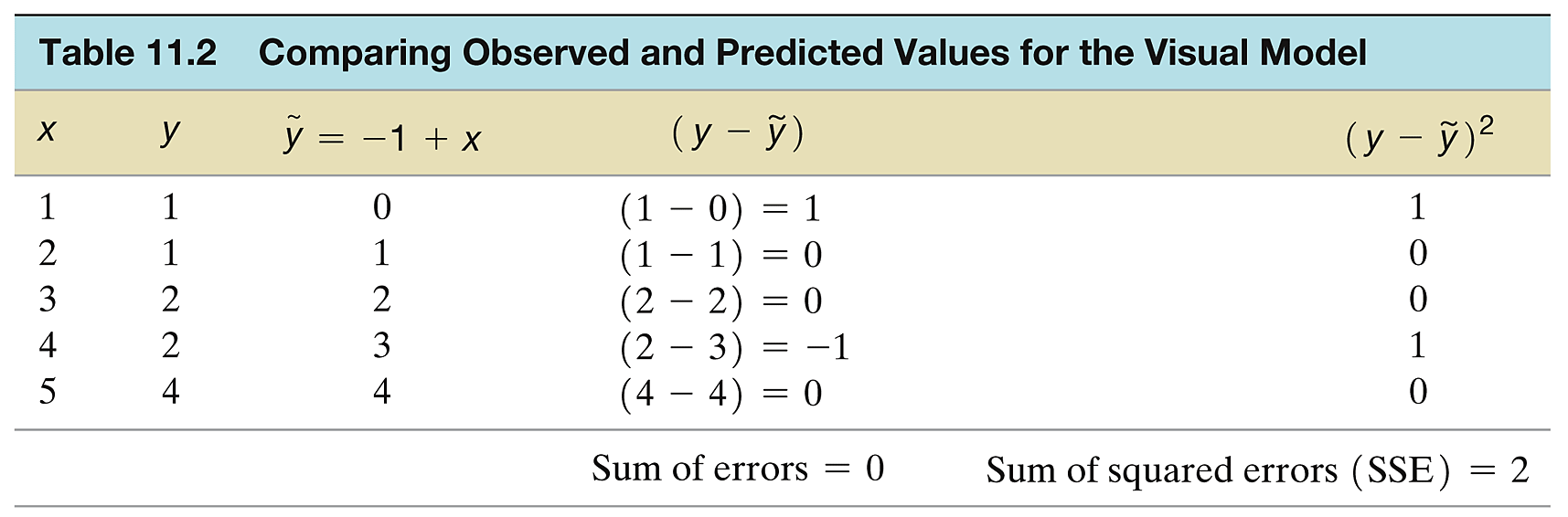
This step is the subject of this section - namely, how can we best use the information in the sample of five observations in Table 11.1 to estimate the unknown \(y\)-intercept \(\beta_0\) and slope \(\beta_1\) ?
# Define the datax <-c(1, 2, 3, 4, 5)y <-c(1, 1, 2, 2, 4)# Create a dataframedata <-data.frame(x, y)# Fit a linear modelmod <-lm(y ~ x, data = data)summary(mod)
Call:
lm(formula = y ~ x, data = data)

Residuals:
         1          2          3          4          5
 4.000e-01 -3.000e-01 -5.551e-17 -7.000e-01  6.000e-01

Coefficients:
            Estimate Std. Error t value Pr(>|t|)
(Intercept)  -0.1000     0.6351  -0.157   0.8849
x             0.7000     0.1915   3.656   0.0354 *
---
Signif. codes:  0 '***' 0.001 '**' 0.01 '*' 0.05 '.' 0.1 ' ' 1

Residual standard error: 0.6055 on 3 degrees of freedom
Multiple R-squared:  0.8167,    Adjusted R-squared:  0.7556
F-statistic: 13.36 on 1 and 3 DF,  p-value: 0.03535
library(ggplot2)ggplot(data, aes(x = x, y = y)) +geom_point() +# Add pointsgeom_smooth(method ="lm", se =FALSE) +ggtitle("Linear Model Fit") +theme_minimal()
You are provided with a dataset of study hours and GPA scores from 15 students. Your task is to input this data into a Shiny app to calculate the correlation, slope, and intercept of the regression line. Analyze these parameters to understand how study hours relate to GPA.
Study Hours (X)
GPA (Y)
1
2.1
2
2.4
3
2.6
4
3.0
5
3.1
6
3.2
7
3.3
8
3.6
9
3.9
10
3.7
11
3.7
12
3.7
13
3.9
14
3.8
15
3.9
Input the Data: Enter the study hours and GPA into the Shiny app.
Calculate the Parameters: Use the app to find the correlation, slope, and intercept.
Interpret the Results:
Correlation: Discuss what the correlation coefficient tells you about the relationship between study hours and GPA.
Slope: Explain what the slope indicates about the effect of an additional hour of study on GPA.
Intercept: Consider the meaning of the intercept in the context of GPA prediction when no study hours are recorded.