Day 41

Math 216: Statistical Thinking
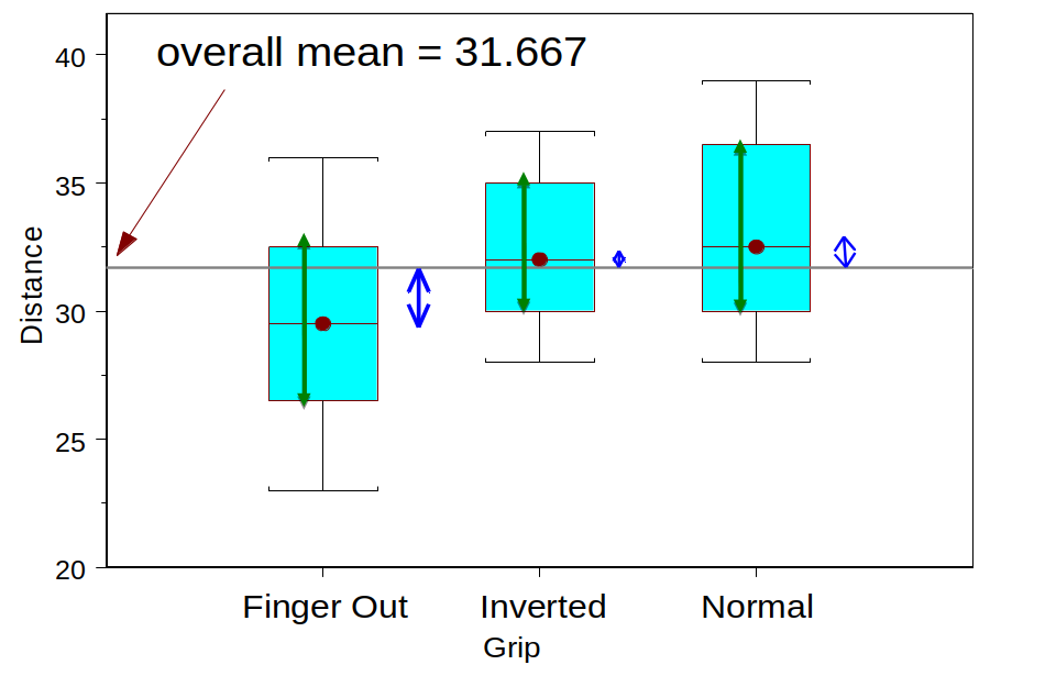
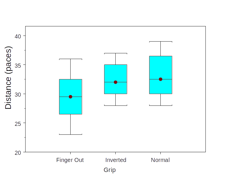
Bastola

Advanced Inference tools

Quantitative Response Analysis:

  • One Mean: Employ 1-sample t-test or confidence interval.
  • Two Means: Use 2 independent sample t-tests/CI or Matched pairs analysis.
  • Multiple Means: Implement One-way ANOVA for comparing more than two groups.

Hypothesis Testing Across Multiple Categories:

\[\begin{align*} H_{0}:& \quad \mu_{1}=\mu_{2}=\ldots=\mu_{k}\\ H_{a}:& \quad \text{At least one } \mu_{i} \neq \mu_{j} \end{align*}\]

Frisbee Example

Does Frisbee grip affect the distance of a throw?

A student performed the following experiment: 3 grips, 8 throws using each grip

1. Normal grip
2. One finger out grip
3. Frisbee inverted grip

A grip type is randomly assigned to each of the 24 throws she plans on making

  • Response: measured in paces how far her throw went
  • Question: How might you summarize her data?

Frisbee Example


  Finger-out Inverted Normal
n 8 8 8
Mean 29.5 32.375 33.125
SD 4.175 3.159 3.944

Question: Is this evidence that grip affects mean distance thrown? \[\begin{align*} H_{0}:& \quad \mu_{1}=\mu_{2}=\mu_{3}\\ H_{a}:& \quad \text{At least one } \mu_{1}, \mu_{2}, \mu_{3} \text{ is not the same} \end{align*}\]

Analyzing Variability in Group Means

Dataset Differences: Although Datasets \(A\) and \(B\) have identical group means, their variability differs significantly.

Mean Variability: Contrasting Datasets \(A\) and \(C\), both showcase similar variability yet differ in group means.

Evidence of Variance: Dataset \(A\) shows minimal evidence of mean differences, whereas Datasets \(B\) and \(C\) display substantial evidence.


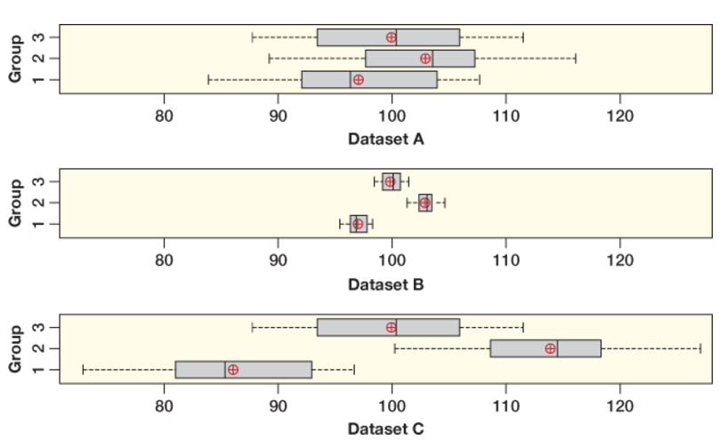
Fig 1: Comparative analysis of group means and variability.

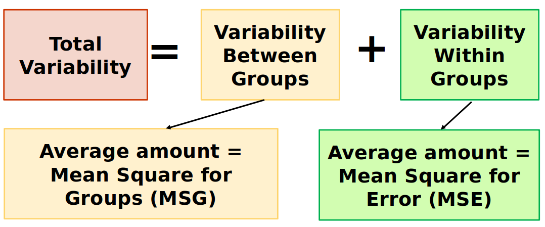
Implications of Variability Analysis

Assessment Criteria: Evaluating differences in means involves:

  • Magnitude of mean differences among groups.
  • Intra-group variability.

Conclusion: A robust analysis of variability is crucial to accurately identify and interpret differences in group means.


Fig 2: Visual evidence supporting variability analysis.

Analysis of Variance

Analysis of Variance (ANOVA) compares the variability between groups to the variability within groups

F-Statistic

The F-statistic is a ratio: \[F=\frac{M S G}{M S E}=\frac{\text { average between group variability }}{\text { average within group variability }}\]

If there really is a difference between the groups \((H_a \text{ true})\), we would expect the F-statistic to be

a). Large positive

b). Large negative

c). Close to 0

Frisbee Example

frisbee <- read.csv("https://raw.githubusercontent.com/deepbas/statdatasets/main/Frisbee.csv")
frisbee.anova <- aov(Distance ~ Grip, data = frisbee) # fit an ANOVA model


summary(frisbee.anova)
            Df Sum Sq Mean Sq F value Pr(>F)
Grip         2  58.58   29.29   2.045  0.154
Residuals   21 300.75   14.32               

F-test statistic: 2.045

P-value: 0.154

F-Distribution

We can use the F-distribution to generate a p-value if:

  1. Sample sizes in each group are large (each \(n_{i} \geq 30\) ) OR the data within each group are relatively normally distributed
  2. Variability is similar in all groups
  • The F-distribution has two degrees of freedom, one for the numerator of the ratio \((\boldsymbol{k}-\mathbf{1})\) and one for the denominator \((n-k)\)
  • For F-statistics, the p-value (the area as extreme or more extreme) is always the right tail

Check assumptions: normality

table(frisbee$Grip)  # check n's

Finger Out   Inverted     Normal 
         8          8          8 

Small \(n_i\) but all groups are roughly normal

# checking normality with qq-plots
ggplot(frisbee, aes(sample = Distance)) + 
  geom_qq() + geom_qq_line() +  facet_wrap(~Grip) +  
  theme(axis.text.x = element_text(size = 4))

Check Assumptions: Equal Variance

The F-distribution assumes equal within group variability for each group. This is also an assumption when using the randomization distribution.

  • As a rough rule of thumb, this assumption is violated if the largest group standard deviation is more than double the smallest group standard deviation
tapply(frisbee$Distance, frisbee$Grip, sd)
Finger Out   Inverted     Normal 
  4.174754   3.159453   3.943802 

Ensure:

\(\frac{\text{largest }s}{\text{smallest }s} < 2\)

Frisbee Example: Inference

Question: Is this evidence that grip affects mean distance thrown?

\[\begin{align*} H_{0}:& \quad \mu_{1}=\mu_{2}=\mu_{3}\\ H_{a}:& \quad \text{At least one } \mu_{1}, \mu_{2}, \mu_{3} \text{ is not the same} \end{align*}\] \(\mu_{\mathrm{i}}\) is the true mean distance thrown using grip \(i\). \[F=2.05(\mathrm{df}=2,21), \text {p-value}=0.1543\]

  • An F-statistic as large as 2.045 would occur by chance about 16% of the time if the means were all equal.
  • Conclusion: Do not reject the Null hypothesis. The difference in observed means is not statistically discernible.

Picturing the variation

Green: Variation within groups

Blue: Variation between groups


ANOVA Table for Frisbee data

\[\text{F-test stat} = 29.29/14.32 = 2.045\]

Source df Sum of Squares Mean Square
Groups
 
#groups -1
3-1 = 2
SSG
58.583
SSG/df
58.583/2 = 29.29
Error
(residual)
n - #groups
24-3 = 21
SSE
300.750
SSE/df
300.75/21= 14.32
Total n-1
24-1 = 23
SSTotal
359.333
 

ANOVA Table formula (don’t memorize!)


Source df Sum of Squares Mean Square
Groups \( k - 1 \) \( \sum_{\text{groups}} n_i (\bar{x}_i - \bar{x})^2 \) \( \frac{SSG}{k - 1} \)
Error (residual) \( n - k \) \( \sum_{\text{groups}} (n_i - 1) s_i^2 \) \( \frac{SSE}{n - k} \)
Total \( n - 1 \) \( \sum_{\text{values}} (x_i - \bar{x})^2 \)